Seeing Through Walls: WiFi Human-Activity Recognition on the Versal AI Engine
A weekend hardware/software co-design that streams WiFi Channel-State-Information (CSI) from a Raspberry Pi into an AMD Versal VCK190, parses the UDP/CSI packets in the Programmable Logic, and runs the STFT + activity / breathing / fall feature extraction on the AI Engine array — turning ordinary WiFi into a device-free room sensor. Validated bit-accurate on real silicon.
My ECE Master's at Mississippi State University was in software-defined-radio (SDR) based sensing. One project asked a deceptively simple question: can an ordinary WiFi signal tell what a person is doing in a room?
The answer is yes — and it comes from Channel-State-Information (CSI). Every OFDM WiFi receiver estimates how the channel distorted each subcarrier. When a body moves, the multipath reflections change, and those changes carry a signature of the motion. I built a WiFi-CSI human-activity recognition (HAR) pipeline, benchmarked it against a radar sensing baseline for accuracy, and published the results across several papers (see Publications).
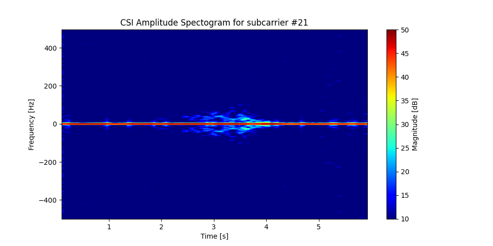
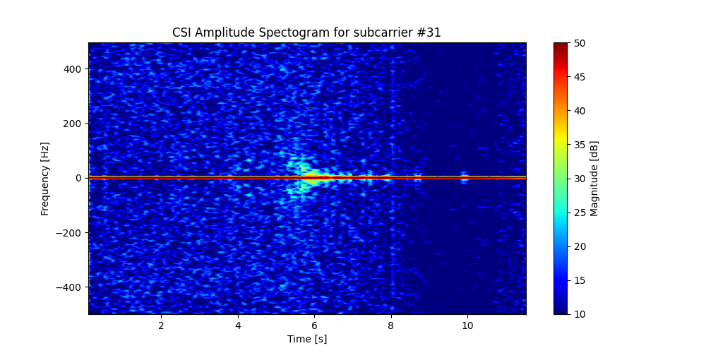
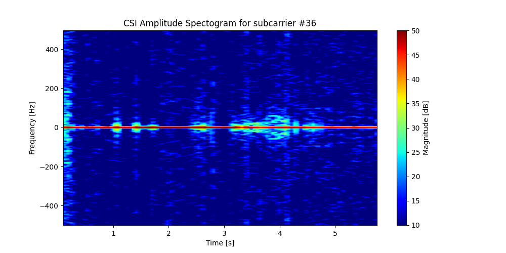
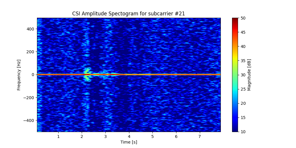
The visual heart of that work is the spectrogram: take the Short-Time Fourier Transform of the CSI time series and each activity paints a distinct time–frequency fingerprint. These are real CSI spectrograms from the dataset — one per activity class:
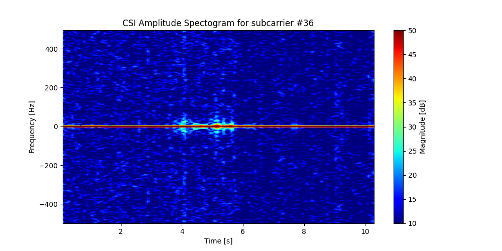
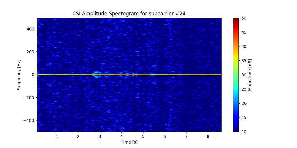
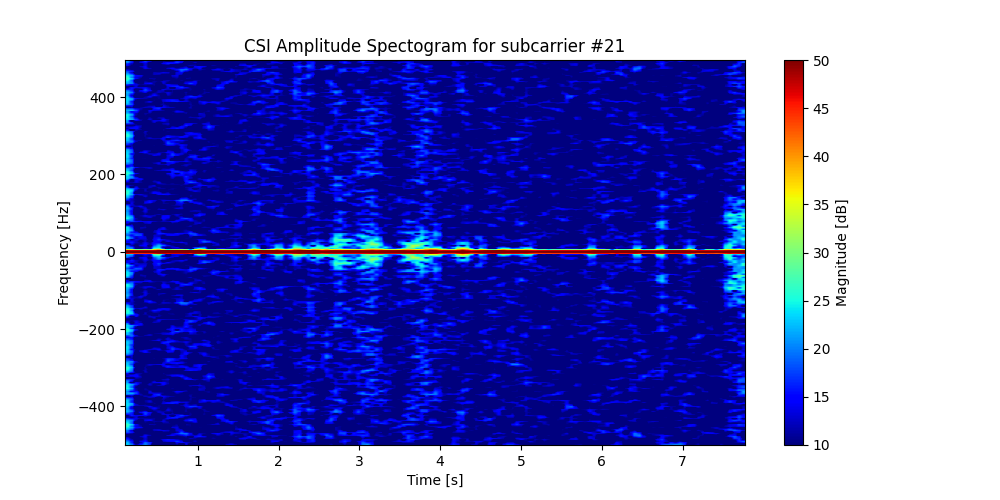
When I presented that thesis to a former manager, they gently suggested that the whole pipeline could, one day, run in an FPGA — the packet parsing in fabric, the heavy DSP and inference on an accelerator. It was said kindly, almost in passing. But it lodged in my head as a personal challenge I promised myself I'd take on someday.
The napkin sketch of that idea looked like this:
The idea sat on the shelf while life moved on. What finally unblocked it was hardware and time: a VCK190 on the bench and a run of weekends and evenings. Modern tooling — and, honestly, LLMs for grinding through the deep Versal tool-flow issues — made a solo build of this scope tractable.
Master's thesis
- WiFi-CSI human-activity recognition
- benchmarked against radar
- published papers
The challenge
- a gentle "do it in an FPGA"
- filed away as a someday goal
Shelved
- other priorities
- idea kept warm
VCK190
- PL UDP/CSI parser
- AIE feature graph
- bit-accurate on silicon
The pipeline now runs on real hardware. A Raspberry Pi running the nexmon_csi firmware patch turns its WiFi chip into a CSI sensor and packetizes CSI as UDP over Ethernet. That stream enters the VCK190 over an SFP link; the PL parses the UDP/CSI packet and streams the I/Q samples straight into the AI Engine, which computes the motion, breathing and phase-variance features. Only the compact results cross into Linux on the Arm cores, where an on-board web dashboard renders what's happening in the room.
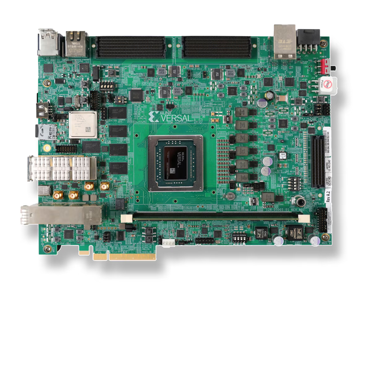
Why this device is the right fit:
- PL streams and parses the Ethernet/UDP packet at line rate.
- The AI Engine is a vector-VLIW array built for FFTs and MAC-heavy DSP — exactly the CSI workload.
- The NoC + DDR and Arm PS handle results and visualization.
- It's a single-chip edge sensor: no PC in the loop.
The full path from WiFi chip to browser. Raw CSI (hundreds of KB/s) never touches the CPU in the target design — only the tiny feature/label vector is DMA'd to Linux. Click any diagram to open it fullscreen and zoom / pan.
bcm43455c0"] --> CAP["CSI extractor"] --> UDP["UDP packetizer"] end UDP -->|"UDP/IP over 1000BASE-X"| SFP["SFP0"] subgraph VCK190["AMD Versal VCK190"] SFP --> GT["GTY + PCS/PMA"] --> MAC["Ethernet MAC"] MAC --> P["PL: csi_udp_parser
strip UDP → I/Q stream"] P --> MUX["csi_mux"] --> AIE subgraph AIE["AI Engine — feature_graph"] FIR["FIR band-pass"] --> ST["stats
mean / var / power"] DFT["windowed-DFT
STFT magnitude"] PH["phase-var
stats"] end AIE --> S2MM["s2mm DMA"] --> DDR[("DDR4 via NoC")] DDR --> A72["Arm A72 · PetaLinux"] A72 --> DASH["live_dashboard.py
SSE web UI"] end DASH --> BROWSER["any browser on the LAN"]
No camera, no wearable, often through a wall. The trick is that your body is part of the radio channel. Here is the intuition, in four steps.
1. CSI is the channel's fingerprint
An OFDM receiver estimates, per subcarrier k, a complex response — amplitude and phase of how the signal arrived. nexmon_csi exposes this vector every packet.
2. You perturb the multipath
The receiver sums many rays: line-of-sight plus reflections off walls, furniture — and you. Move, and the reflected path length changes, rotating its phase and reshaping the summed H[k] over time.
3. Motion → Doppler
A body part moving at velocity v imparts a Doppler shift. Different activities have different velocity signatures, so the STFT separates walking from falling from sitting.
4. Breathing → slow phase tone
The chest wall moves millimeters at ~0.2–0.4 Hz. That appears as a narrow low-frequency tone in the CSI — the basis of the breathing branch.
Why STFT. Activities are non-stationary, so we take the Short-Time Fourier Transform of the CSI time series — window, DFT, magnitude — producing the time–frequency spectrograms you saw in Act 1. (This directly builds on my paper Effect of the Short-Time Fourier Transform on the Classification of Complex-Valued Mobile Signals.)
WiFi vs. radar — the thesis comparison
Radar is dedicated, high-bandwidth and precise, but it's extra hardware. WiFi CSI reuses ubiquitous infrastructure: it's device-free, works in the dark and through walls, and is privacy-preserving (no imagery). My thesis and our RadarConf 2024 paper comparing Wi-Fi-CSI and radar-based HAR quantified that accuracy trade-off — the motivation for pushing the WiFi pipeline all the way onto an edge accelerator here.
In the target architecture the PL owns the packet. RX frames enter as an AXI4-Stream; a
custom csi_udp_parser (Vitis HLS)
filters the CSI UDP port, strips the Ethernet/IP/UDP headers, extracts the I/Q payload, and streams samples
through a csi_mux straight into the
AI Engine. This is the real Vivado block design that was built and run on the board:
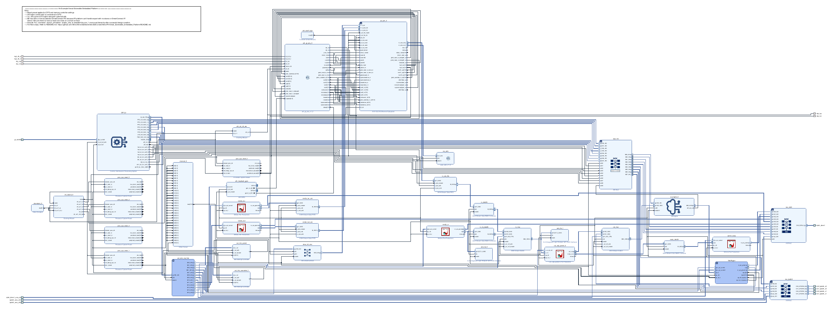
csi_udp_parser → csi_mux → ai_engine → s2mm DMA → NoC → DDR4. Exported with write_bd_layout from the built project.A simplified view of the same PL datapath, for reference:
(width conv.)"] RXW --> PAR["csi_udp_parser
(HLS)"] PAR --> MUX["csi_mux"] MUX --> SHIM["AIE ↔ PL shim
(v++ co-generated)"] SHIM --> AIE["ai_engine_0"] AIE --> S2MM["s2mm"] --> NOC["NoC"] --> DDR[("DDR4")]
Under the hood the parser is a one-byte-per-cycle state machine (Vitis HLS,
II=1): it walks each Ethernet frame byte by byte, checks a handful of fixed offsets to accept or
drop the frame, and reassembles the little-endian int16 I/Q payload into 32-bit words. The whole
wire contract is just these offsets:
| Byte(s) | Field | Parser action |
|---|---|---|
12–13 | EtherType | keep only 0x0800 (IPv4) |
23 | IP protocol | keep only 17 (UDP) |
36–37 | UDP dest port | keep only the CSI port (5500) |
44 | nexmon RSSI | int8 dBm → metadata |
52–53 | sequence no. | → metadata (packet-loss tracking) |
54 | core / spatial | → metadata |
56–57 | chanspec | channel + bandwidth → metadata |
60 → | CSI payload | int16 LE real, then imag, per subcarrier (up to 256) |
The complex pair. From byte 60 the parser takes four wire bytes at a time — two for the real
part, two for the imaginary — sign-extends each int16, and packs them into one 32-bit AXI4-Stream
beat. That packed word is the complex CSI sample H[k] = I +
jQ for a single subcarrier:
// CSI payload from byte 60: int16 LE real, int16 LE imag.
ap_int<16> re; re(7,0) = b0; re(15,8) = b1;
ap_int<16> im; im(7,0) = b2; im(15,8) = b;
axis_csi o;
o.data(15,0)  = (ap_uint<16>)re;   // real -> low half
o.data(31,16) = (ap_uint<16>)im;   // imag -> high half
o.last = beat.last;                 // TLAST marks end-of-CSI for this frame
csi_out.write(o);                   // one 32-bit beat per subcarrier
n_sub++;
So the parser emits two synchronized AXI4-Streams per WiFi frame: csi_out, the run
of complex subcarriers, and meta_out, a single 64-bit record carrying everything the downstream
needs to normalize and label the window:
| Stream | Width | Payload |
|---|---|---|
csi_out | 32-bit | { imag[31:16], real[15:0] } × up to 256 subcarriers |
meta_out | 64-bit | { seq, rssi, n_sub, chanspec, core_spatial } — one packed record per frame |
1 B / cycle · TLAST = frame"] --> FILT{"IPv4? · UDP?
port 5500?"} FILT -->|"no"| DROP["discard frame"] FILT -->|"yes"| HDR["latch header bytes
44 · 52 · 54 · 56"] HDR --> ASM["reassemble int16 I/Q
from byte 60"] ASM --> CS["csi_out
32-bit complex
{imag, real}"] HDR --> MT["meta_out
64-bit record
seq·rssi·n_sub·chanspec"]
The whole parser costs about 1.3% of the PL LUTs, zero DSPs and a few BRAMs — line-rate protocol offload is exactly what the fabric is cheapest at, which is why it lives here and not on the Arm.
The parser produces per-packet complex vectors, but the AI Engine branches want real-valued time windows — a stretch of many packets for one subcarrier. Bridging the two is a short conditioning chain, and deciding where each step runs — PL, AI Engine, or Arm — is the heart of the hardware/software co-design.
per subcarrier"] --> AP["magnitude / phase
via CORDIC"] AP --> SAN["phase sanitize
linear de-trend"] SAN --> SEL["subcarrier select
variance top-K"] SEL --> WIN["window / ring-buffer
L=256 · N=64"] WIN --> AIE["→ AI Engine branches"]
Magnitude feeds the motion and breathing branches; phase feeds the phase-var branch. Phase first gets a per-packet linear de-trend across subcarriers, which cancels the carrier-frequency offset (the intercept) and the sampling/packet-delay offset (the slope) that otherwise swamp the real motion:
Where each stage of the pipeline lands is a deliberate partitioning decision:
| Stage | Runs on | Why there |
|---|---|---|
| UDP/CSI parse · I/Q depacketize | PL | cheap streaming bit-manipulation at line rate |
| |H| / ∠H (CORDIC) | PL | CORDIC is a fabric primitive |
| phase sanitize · FFT / STFT · FIR | AI Engine | vectorized float MACs and butterflies |
| subcarrier select · windowing | PL + DDR | light control logic + data movement |
| thresholds · labels · dashboard | Arm A72 | control plane and UX |
Rule of thumb across the whole design: streaming & bit-twiddling → PL; FFT / GEMM / filters → AI Engine; control & UX → the Arm.
Those three conditioned windows are exactly what the graph waits on — each lands on its own PLIO stream input, and from here the whole pipeline stays on the AI Engine array. It runs a three-branch feature graph, one branch per window: the two amplitude windows drive motion and breathing, while the sanitized-phase window drives phase-var.
Each branch maps directly to a piece of the physics above, and every kernel is a small streaming function connected window-to-window over PLIO:
amplitude · 256"] --> FIR["kfir: FIR band-pass"] --> STA["kstats: mean/var/power"] --> O1["PLIO_out
motion {mean,var,power}"] BIN["PLIO_brt_in
amplitude · 64"] --> DFT["kdft: windowed-DFT magnitude"] --> O2["PLIO_brt_out
NB breathing bins"] PIN["PLIO_phase_in
phase · 256"] --> PHA["kphase: stats"] --> O3["PLIO_phase_out
phase-var {mean,var,power}"]
| Branch | Kernel chain | Output | Physical meaning |
|---|---|---|---|
| Motion | FIR band-pass → stats | {mean, var, power} | band-limit to the human-motion Doppler band, then measure energy → presence / activity intensity |
| Breathing | windowed-DFT magnitude | NB bins | STFT bin near 0.2–0.4 Hz → respiration rate |
| Phase-var | stats | {mean, var, power} | phase variance → micro-motion / stability, feeds fall detection |
Why three? Human activity shows up in the CSI at three different mechanisms and time-scales at once, so each branch is tuned to one of them and they run in parallel on separate AI Engine tiles:
Motion — fast amplitude
A 31-tap band-pass FIR keeps only the ~1–3 Hz human-Doppler band of a 256-sample amplitude window; stats then reports its variance / power. High energy means someone is moving.
Breathing — slow periodic
A 64-point Hann-windowed DFT turns a slow amplitude window into 33 magnitude bins; the peak in the 0.1–0.5 Hz band is the respiration tone (6–30 breaths/min).
Phase-var — micro-motion
After sanitization, the variance of the phase over a 256-sample window is a scale-immune presence cue — it survives when amplitude is ambiguous, and it feeds fall detection.
The graph wiring is pure ADF — kernels connected stream-to-stream on the array:
// motion branch: FIR band-pass -> stats (kernel-to-kernel)
connect<>(in.out[0],    kfir.in[0]);
connect<>(kfir.out[0],  kstats.in[0]);
connect<>(kstats.out[0], out.in[0]);
// breathing branch: windowed-DFT magnitude
connect<>(brt_in.out[0], kdft.in[0]);
connect<>(kdft.out[0],   brt_out.in[0]);
// phase-variance branch: stats -> variance is the phase-var feature
connect<>(phase_in.out[0], kphase.in[0]);
connect<>(kphase.out[0], phase_out.in[0]);static inline void stats_core(const float *x, float *out) {
float s = 0.0f;
for (int i = 0; i < L; i++) s += x[i];
float mean = s / (float)L;
float sd = 0.0f, s2 = 0.0f;
for (int i = 0; i < L; i++) {
float d = x[i] - mean;
sd += d * d;
s2 += x[i] * x[i];
}
out[0] = mean; // DC / bias
out[1] = sd / (float)L; // variance == motion-band / phase-var energy
out[2] = s2 / (float)L; // power
}
Per window the three branches emit 39 floats — mot[3], brt[33],
phs[3]. Together with the RSSI from the parser metadata, those collapse into the compact
8-feature vector the classifier actually consumes:
| # | Feature | Where it comes from |
|---|---|---|
0 | presence | motion + phase-var vs. threshold |
1 | motion | motion-branch variance / power |
2 | breathing (bpm) | breathing-branch peak DFT bin |
3 | heart rate | reserved (unreliable at 20 Hz CSI) |
4 | phase-var | phase-var-branch variance |
5 | persons | classifier |
6 | fall | motion transient + debounce |
7 | RSSI | parser metadata, (rssi+100)/100 |
{mean,var,power}"] --> V["8-feature
vector"] B["breathing
33 DFT bins"] --> V P["phase-var
{mean,var,power}"] --> V R["RSSI (metadata)"] --> V V --> MLP["pretrained MLP
8→64→128 · L2"] --> LBL["activity label
+ presence / vitals"]
The classifier is deliberately tiny — a pretrained 8→64→128 MLP (~9k parameters, GELU + batch-norm, L2-normalized embedding) plus a linear presence head. All the heavy lifting is the DSP feature stage above: the vector-VLIW AI Engine chews through the FIR taps and DFT butterflies far faster than the scalar A72 could — which is the whole point of the offload.
The subtle bug that cost the most: the AIE ↔ PL shim
A plain Vivado block design that wires a PL stream into the AI Engine's S00_AXIS stalls on
silicon — TREADY never asserts. The reason: a hand-built BD does not emit the paired AIE↔PL
shim solution that the graph's PLIO placement requires. The binding must be co-generated by
v++ --link. The fix inserts the PL stream on v++'s own post-SysLink block design via an
overlay hook, leaving ai_engine_0 untouched so the correct shim solution is preserved.
The last hop is deliberately thin. Two s2mm data movers — one for the AI Engine features, one for the
parser metadata — are PL AXI-MM masters that push their results across the Versal NoC into a small
reserved region of DDR4. The Arm A72 running PetaLinux reads that region and serves the dashboard. The
multi-hundred-KB/s raw CSI stream never crosses into Linux — only a few hundred bytes of features
and metadata per window do.
39 floats / window"] --> S["s2mm"] METAI["parser metadata"] --> SM["s2mm_meta"] S --> NOC["Versal NoC"] SM --> NOC NOC --> DDR[("DDR4
reserved no-map
@ 0x7000_0000")] DDR --> A72["Arm A72
PetaLinux"] A72 --> DASH["live_dashboard.py
SSE web UI"]
Because s2mm and s2mm_meta are driverless PL masters with no IOMMU, they write to a 1 MB
no-map carve-out that Linux does not own: the packed metadata record sits at the base and the feature
results 64 KB in, so the two never share a page. Everything is memory-mapped at fixed addresses that the on-target
control tool (sw/csi_ctl.c — mac-init, start, mux,
meta) and the reader agree on:
| Block | AXI base |
|---|---|
mm2s — DDR → AIE (golden path) | 0xA400_0000 |
s2mm — AIE features → DDR | 0xA401_0000 |
csi_udp_parser | 0xA402_0000 |
s2mm_meta — metadata → DDR | 0xA403_0000 |
csi_mux — AXIS switch | 0xA406_0000 |
ethernet MAC | 0xA408_0000 |
ai_engine | 0x20_0000_0000 |
The csi_mux is what makes both worlds testable: flip it one way and the AI Engine is fed by the live
Ethernet parser; flip it the other and it's fed by mm2s replaying a known CSI window from DDR — the
bit-exact golden test that anchors every silicon bring-up below.
Talk is cheap — here is the datapath caught in the act on a real VCK190 (board chanterelle10). Four ILA taps were inserted on the live pipeline via the Versal debug automation: ETH_RX (nexmon UDP bytes), CSI_PARSED (parser output), AIE_IN (mux → AI Engine) and AIE_OUT (AIE features → DMA).
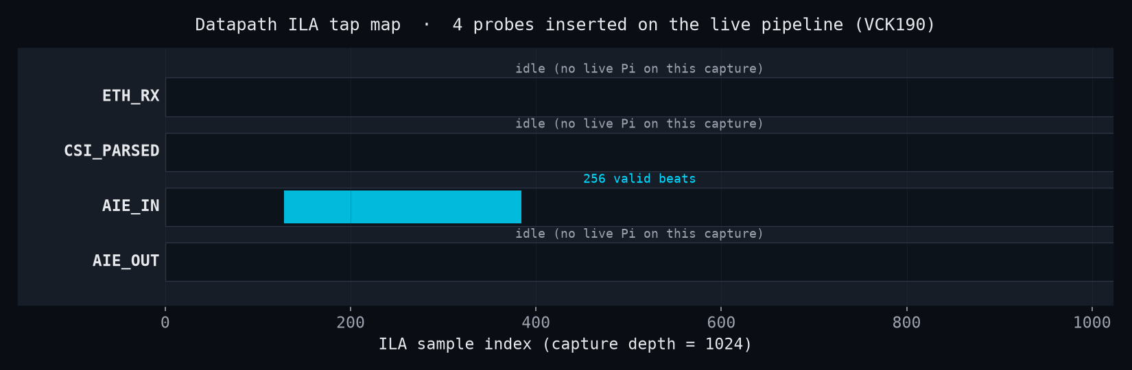
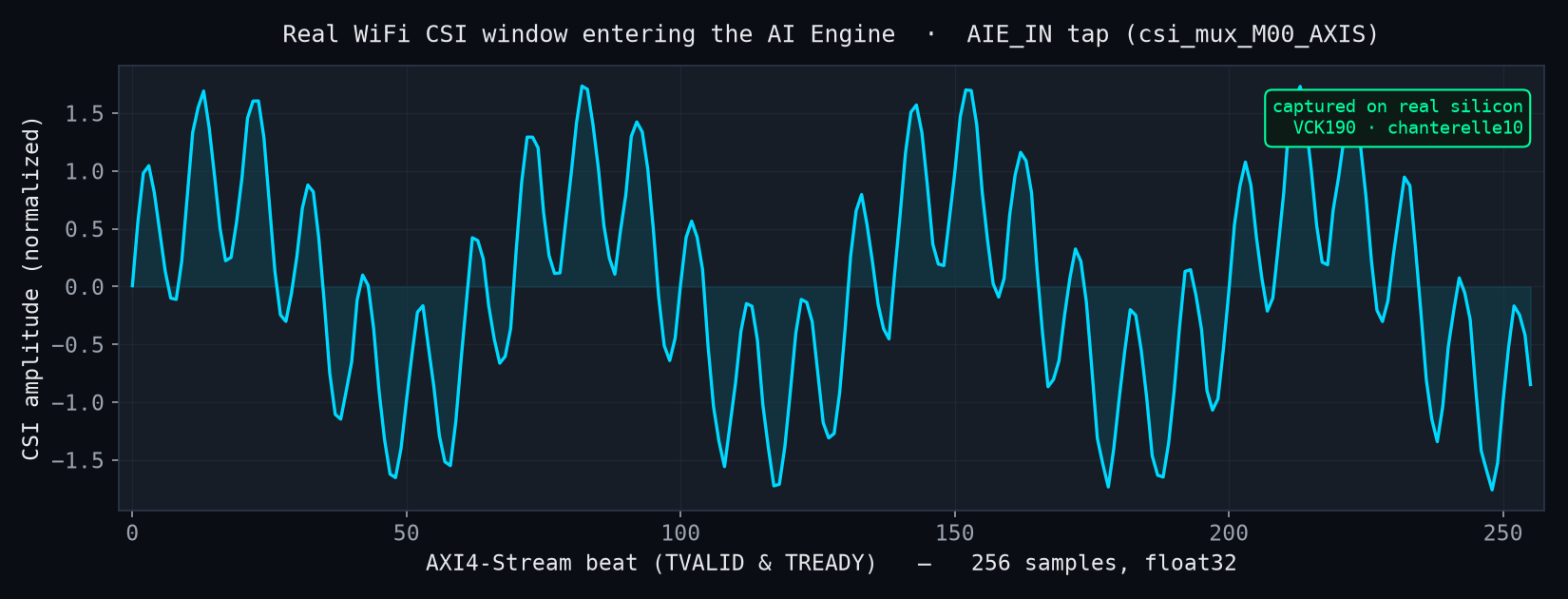
0x3f0ec77a = 0.558).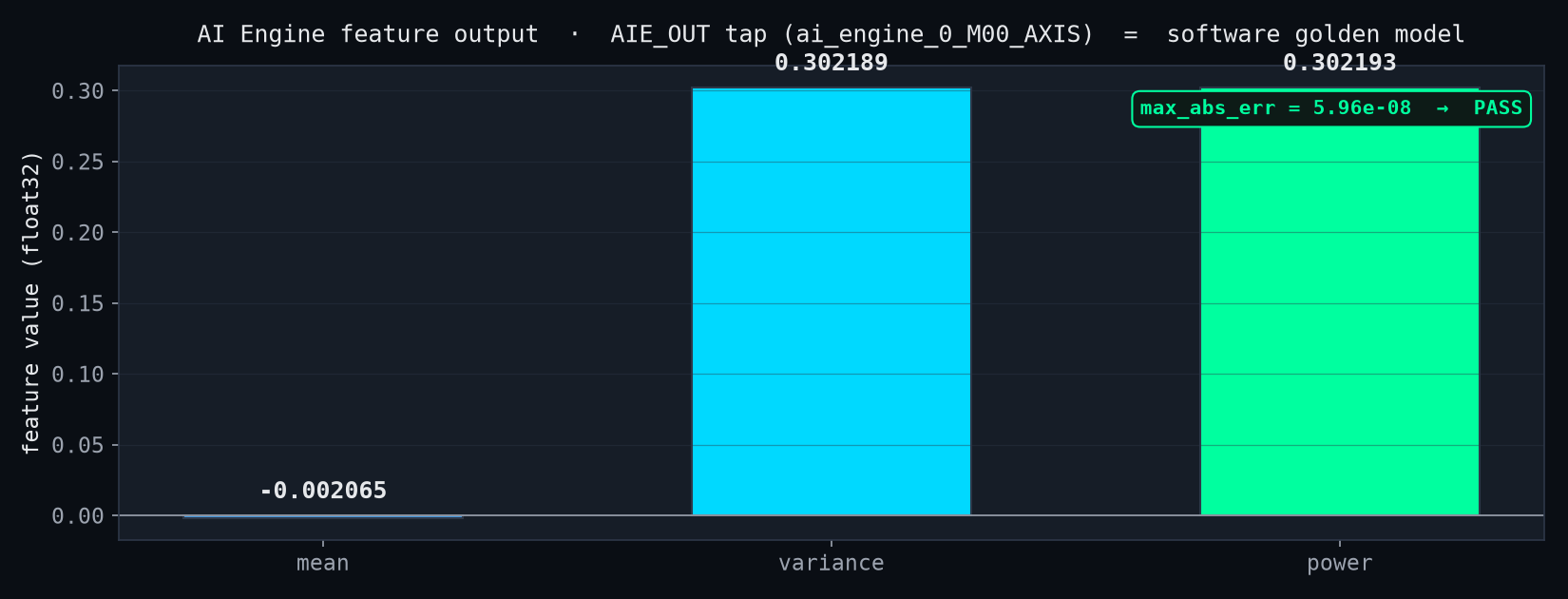
The end-to-end numerical check, on hardware:
The VCK190 serves its own dashboard (pure-Python, standard-library only, no CDN — it runs on a bare
PetaLinux rootfs). It consumes the AI Engine feature groups and derives presence, activity, breathing rate
and fall alerts — and renders a live CSI spectrogram by stacking the streamed
brt[33] windowed-DFT magnitude vectors over time (the same STFT view from Act 1, now updating in
real time). Below is that dashboard's logic, replaying a representative feature stream right in your
browser — empty room → someone walks in → sits and breathes → a fall → stillness:
The widget above is a representative feature-stream replay running the same metrics and thresholds as the on-board dashboard — it is not a live capture. On the board, these tiles update from live AI-Engine features.
A full live demo — Raspberry Pi streaming CSI into the VCK190, the room being sensed in real time — is being recorded. Until then, the interactive dashboard above is the teaser.
The gap between "works in simulation" and "works on silicon" was where the real engineering happened. A few that cost days:
The AIE ↔ PL shim must be co-generated by v++
S00_AXIS stalls — TREADY never asserts — because it lacks the v++-generated shim solution (aieshim_solution.aiesol / aie_pl_intf.json) the PLIO placement requires. Fix: insert the PL stream on v++'s own post-SysLink BD through an overlay hook, leaving ai_engine_0 untouched. The resulting XSA carries the full shim solution and the DDR → mm2s → AIE → s2mm → DDR stream is bit-accurate on silicon.The debug build crashed the placer — an unplaced GT quad
place_design in "Phase 5.1 Post Place Optimization". Root cause wasn't the ILAs alone: the co-generated Ethernet GT quad was left unplaced (the external SFP ports aren't top-level accessible under v++, and the OOC gt_quad can't be LOC'd from a top XDC). Fix: an implementation OPT_DESIGN.TCL.POST hook (gtloc_hook.tcl) LOCs the leaf cells after link — quad_inst → GTY_QUAD_X0Y5, IBUFDS_GTE5 → GTY_REFCLK_X0Y10. With both placed, place + route + write_device_image all pass.Three integration fixes to make the AIE actually run under Linux
interrupts-extended (the CU IRQs) to the zocl / zyxclmm_drm device-tree node; (2) bake the aie_image graph CDO into BOOT.BIN; (3) drop graph.wait() in the host, because the packaged CDO free-runs the graph — you drain s2mm instead.The Ethernet image boots — it was a timing race, not a dead board
Image / boot.scr / dtb / rootfs, then booti. With that, the eth image boots Linux 6.12.40 and its ILAs capture live data end-to-end.| Layer | Technology | Role |
|---|---|---|
| CSI source | Raspberry Pi + nexmon_csi | WiFi NIC → per-packet CSI → UDP |
| Link | 1000BASE-X SFP | Pi Ethernet → VCK190 GTY |
| Device | AMD Versal VCK190 | PS (A72) + PL + AI Engine ACAP |
| Packet parse | Vitis HLS csi_udp_parser | UDP/CSI depacketize in PL |
| DSP + inference | AI Engine (ADF graph) | FIR / DFT / stats feature extraction |
| Data movement | mm2s / s2mm + NoC + DDR4 | PLIO ↔ DDR, results to PS |
| Tools | Vivado / Vitis 2025.2 | synth, AIE compiler, v++ link |
| Embedded OS | PetaLinux 2025.2 + XRT | A72 Linux, board host app |
| Visualization | Python stdlib SSE dashboard | on-board live web UI |
The research this build stands on. Full profile on Google Scholar.
The whole project is open source. I've deliberately made it turnkey — a single
project_top.tcl rebuilds the Vivado design end-to-end, and the tracked
petalinux/ project directory has everything you need to build the Linux image for the board.
Fully reproducible builds — a standard I hold on every reference design
Reproducibility isn't an afterthought here; it's how I ship. Across all of my reference designs the
entire Vivado project rebuilds from a single tracked TCL script and the
PetaLinux image from a tracked project-spec — no GUI click-throughs, no
undocumented state, so anyone can clone the repo and rebuild it bit-for-bit. You'll find the exact same
discipline in my
Versal Ethernet and
ZCU102 Ethernet
reference designs. It's the same production-grade, source-controlled methodology I apply to the AMD
reference designs I author professionally.
One-command Vivado build
hw/scripts/project_top.tcl conveniently builds the inline Vivado project (Ethernet → csi_udp_parser → AI Engine → DMA) into an XSA end-to-end — no manual block-design wiring.
Ready-to-build PetaLinux
The petalinux/ directory ships the full project-spec/ (recipes + configs), the SDT flow, and the boot / rootfs bring-up scripts — everything needed to build and boot this project on the VCK190.
AIE graph + HLS parser
The AI Engine feature graph (aie/), the Vitis HLS UDP/CSI parser (hls/), the v++ co-generation flow and the on-board dashboard (live/) are all in the repo, with a phase-by-phase build log in docs/.
The Versal pipeline is only as real as the CSI feeding it. The transmitter is a
Raspberry Pi 4B whose Broadcom bcm43455c0 Wi-Fi chip is reflashed with the
nexmon_csi firmware patch: it turns
every received OFDM frame into a per-subcarrier CSI vector and emits it as a
UDP packet on port 5500. A small boot-time service then relays that stream out the Pi's
Ethernet port to the VCK190's SFP.
monitor · ch132/80"] --> FW["CSI firmware
7.45.189 nexmon.org/csi"] FW --> U["UDP :5500 on wlan0
10.10.10.10 → 255.255.255.255"] U --> SVC["csi-forward.service
wlan0 → eth0"] end SVC -->|"UDP/IP · 1000BASE-X SFP"| VCK["VCK190 SFP0 → csi_udp_parser → AI Engine"]
This Pi runs Raspberry Pi OS Trixie on kernel 6.18 — far newer than
nexmon's classic brcmfmac-patch targets — so it uses the maintainer's
recent-kernel path (Makefile.rpi + nl80211 vendor commands, no modified driver).
sudo apt install -y git libgmp3-dev gawk qpdf bison flex make autoconf \
     libtool texinfo xxd libnl-3-dev libnl-genl-3-dev bc libssl-dev tcpdump
sudo dpkg --add-architecture armhf && sudo apt update
sudo apt install -y libc6:armhf libisl23:armhf libmpfr6:armhf libmpc3:armhf libstdc++6:armhf
sudo ln -sf /usr/lib/arm-linux-gnueabihf/libisl.so.23 /usr/lib/arm-linux-gnueabihf/libisl.so.10
sudo ln -sf /usr/lib/arm-linux-gnueabihf/libmpfr.so.6 /usr/lib/arm-linux-gnueabihf/libmpfr.so.4
# the b43 disassembler also needs python2.7 (from the Debian archive)git clone --depth 1 https://github.com/seemoo-lab/nexmon.git && cd nexmon
source setup_env.sh
sed -i '1 s/$/2.7/' $NEXMON_ROOT/buildtools/b43-v3/debug/b43-beautifier
make # extract ucode / flashpatches
cd $NEXMON_ROOT/utilities/nexutil
sudo -E make install USE_VENDOR_CMD=1 # REQUIRED on recent kernels
sudo setcap cap_net_admin+ep /usr/bin/nexutil
cd $NEXMON_ROOT/patches/bcm43455c0/7_45_189
git clone --depth 1 https://github.com/seemoo-lab/nexmon_csi.git && cd nexmon_csi
make -f Makefile.rpi install-firmware && sudo reboot # reboot loads the CSI firmwarenexutil -Iwlan0 -m1 # monitor mode
PARAMS=$(makecsiparams -c 132/80 -C 1 -N 1) # ch132, 80 MHz, core0, ss0
nexutil -Iwlan0 -s500 -b -l34 -v"$PARAMS" # configure the extractor
sudo tcpdump -i wlan0 -nn dst port 5500 # → length-1042 UDP framesEach frame is exactly what the PL csi_udp_parser reads — an 18-byte nexmon header, then 256
int16 I/Q pairs (80 MHz):
| Byte | Field | Captured |
|---|---|---|
42 | magic 0x1111 | — |
44 | RSSI (int8) | −47 dBm |
52 | sequence | per-frame |
54 | core / spatial stream | 0 / 0 |
56 | chanspec | 0xe08a = 132/80 |
60 … | CSI — int16 LE real, int16 LE imag ×256 | 1024 bytes |
📎 Download a real 40-frame CSI capture
(csi_sample.pcap, ch132/80) — the byte offsets above line up 1:1 with
hls/csi_udp_parser.cpp.
The bring-up war-stories — the ones that actually cost time:
The CSI ioctl returned -EBADE — stock firmware was still loaded
update-alternatives, but the driver
had already loaded the stock brcmfmac43455-sdio.bin at boot, so
nexutil -s500 was rejected with -EBADE (which presents as a hang). A
reboot is what makes the driver actually download the CSI firmware
(version 7.45.189 nexmon.org/csi); a plain module reload does not re-flash the chip.nexutil needs -Iwlan0, and must be built with USE_VENDOR_CMD=1
USE_VENDOR_CMD=1 they are rejected, and without an explicit
-Iwlan0 the SET call blocks. An strace confirmed the sequence: vendor command
sent, driver acks, done.Skipping the armhf cross-libs silently kills monitor mode
:armhf libisl/libmpfr under their legacy sonames. Skip the
symlinks and the firmware builds but monitor mode never engages.Boot-time UDP sender (Pi → VCK190)
nexmon injects the CSI onto wlan0 (the monitor interface); it never leaves the Pi on its own.
A stdlib-Python systemd service captures those frames at layer 2 and re-emits the nexmon
payload as a fresh UDP datagram on eth0 — reproducing the exact
ethertype@12 / proto@23 / dport@36 / nexmon@42 / CSI@60 offsets, so the Versal parser gets a
byte-correct frame:
# csi-forward.service runs csi_forward.py:
#   raw AF_PACKET capture on wlan0 (udp/5500)  →  UDP sendto on eth0
sudo systemctl enable --now csi-activate.service csi-forward.service
# on the receiver:  sudo tcpdump -i eth0 -nn udp dst port 5500  → length-1042 frames
Validated live: wlan0 → eth0 at ~470 frames/s
with the byte layout intact.
Status — the last mile
The Pi source and the Ethernet forwarder are done and format-verified against the parser. The Versal live
front-end (GT + MAC + csi_udp_parser + csi_mux) is built in the
v++ co-generation flow; on-silicon bring-up with the Pi over the SFP link — PCS link plus live
parser → AI Engine — is the remaining step.
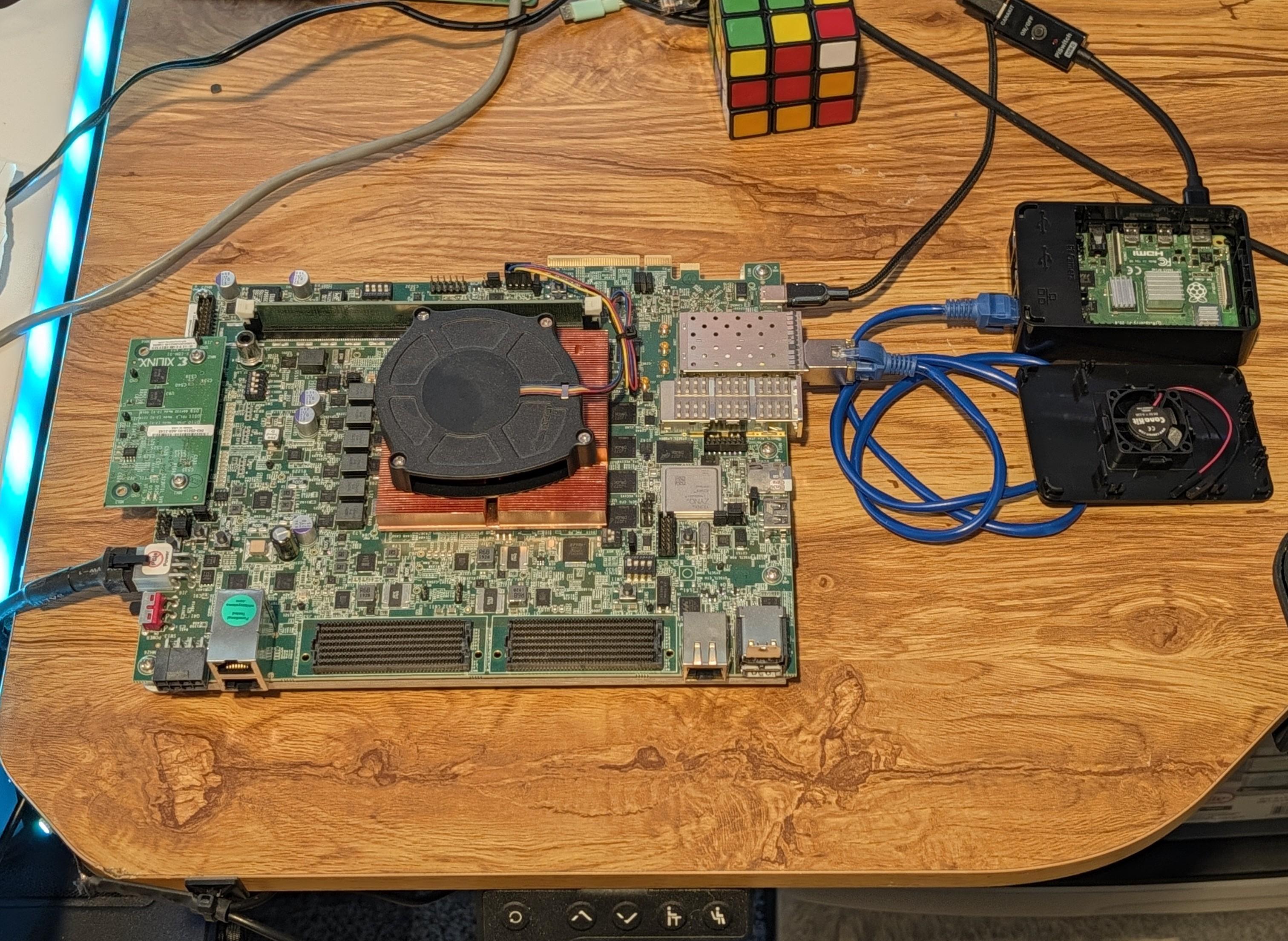
nexmon_csi, streaming CSI over Ethernet to the VCK190.